An AI model trained on tens of thousands of simulated planetary systems achieved up to 99% precision at recognising simulations containing an Earth-mass planet in a broad temperate zone. Applied to 1,567 real systems, it identified 44 priority targets—but whether that extraordinary hit rate survives contact with the real sky remains untested.

The most important word in the reported 99% precision is simulated.

The classifier was not given a group of real planetary systems whose unseen planets were already known independently. It learned from computer-generated systems, and its remarkable precision was measured on other systems produced by the same family of simulations. Only after that test did the researchers apply it to observations.

The result is therefore both interesting and unfinished. It offers astronomers 44 places where follow-up observations may be unusually productive. It does not amount to 44 newly detected Earths, and it does not show that every target has a 99% chance of hiding one.

That boundary is not a minor technical qualification. It is the central question the work has placed before the real sky.

What the study called an Earth-like planet

In their peer-reviewed Astronomy & Astrophysics study, Jeanne Davoult, Romain Eltschinger and Yann Alibert needed a clear label for their machine-learning model. They called the target an “Earth-like planet,” abbreviated ELP.

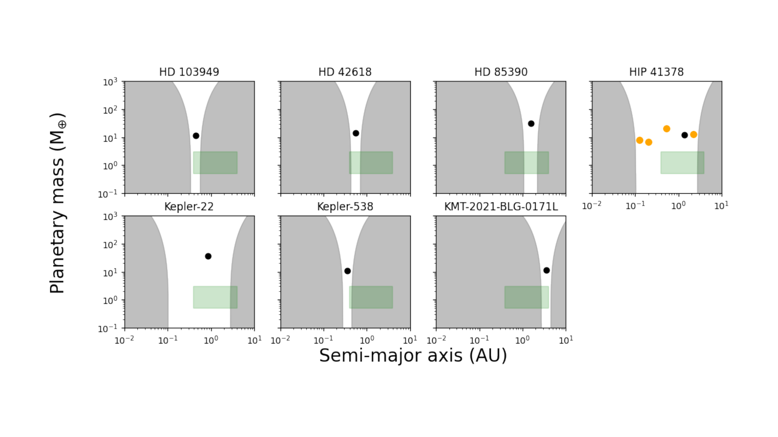
An ELP had to satisfy two conditions. Its mass had to fall between 0.5 and 3 times the mass of Earth, and its equilibrium temperature had to lie between 160 and 510 kelvin, or about minus 113 to 237 degrees Celsius.

The temperature range is deliberately much wider than a conventional habitable zone. Around a star like the Sun, the paper’s zone extends from about 0.39 to 3.9 astronomical units. Around stars with 0.5 and 0.2 solar masses, its outer edges reach roughly 2.52 and 1.48 astronomical units respectively.

The authors chose this broad interval partly to place more positive examples in the training data. That helped reduce the imbalance between systems that did and did not contain a target planet.

It also means “Earth-like” should be read narrowly here. The label says nothing directly about a planet’s radius, rock-to-gas ratio, atmosphere, water, surface pressure, magnetic field or biological potential. It identifies a broad mass-and-temperature class, not another Earth.

A synthetic universe where every planet is known

The researchers trained their model using Generation III of the Bern global model of planet formation and evolution. The Bern framework begins with disks of gas and planetesimals around young stars, follows planetary embryos as they grow and migrate, and then evolves the resulting systems.

For this experiment, the source populations contained 24,365 simulated systems around stars with the Sun’s mass, 14,559 around stars half as massive and 14,958 around stars one-fifth as massive. That is 53,882 generated systems before filtering.

Some contained no surviving planets. Others had no planets above the study’s simplified detection limits. Once those cases were removed, 35,385 systems remained for the three stellar-mass-specific classifiers: 20,365 in the Sun-mass group, 10,158 in the half-Sun group and 4,862 in the lowest-mass group.

A synthetic catalogue gives machine learning an advantage that nature does not. The simulation knows every planet it created, including planets that would be too difficult for present instruments to detect. Each system can therefore be labelled with certainty as containing or not containing an ELP under the paper’s definition.

The scientific wager is that the visible planets retain information about their hidden siblings. If planet formation builds whole systems rather than unrelated worlds, the arrangement of the planets already detected might help predict what remains unseen.

How the team made planets “invisible”

A model trained on complete simulated systems would have little practical value if it could simply read the mass and orbit of the target planet. The researchers therefore masked weaker planets using thresholds based on the radial-velocity wobble they would produce in their stars.

The adopted semi-amplitude limits were 0.43 metres per second for Sun-mass stars, 0.76 metres per second for half-Sun stars and 1.55 metres per second for the smallest stars. The thresholds were selected so that planets within the ELP definition would be hidden from the classifier’s input.

The task was then indirect: infer an unseen ELP from the properties of the planets left above the threshold. In effect, the model was asked to recognise a planetary family from the relatives that current observations might reveal.

The paper is candid that this is a crude version of observational selection. A fixed amplitude limit does not reproduce stellar activity, instrumental noise, the duration and cadence of a survey, the planet’s orbital period, or the difficulty of disentangling several signals in one system.

Those complications matter because the 1,567 real systems did not emerge from a single uniform survey with three clean cutoffs. They were assembled by many telescopes, techniques and observing programmes, each with different blind spots.

What the random forest actually learned

The “AI” in this work was a random-forest classifier, not a large language model or a system that invents planetary descriptions. A forest combines the votes of many decision trees. This one used 500 deliberately shallow trees, each limited to a maximum depth of five and a minimum of 100 samples at a split.

The most useful inputs were surprisingly compact. The model received the architectural class of the planetary system plus the mass and orbital period of its innermost detectable planet. The host star’s mass determined which of the three specialised forests was used.

Planetary architecture is the system-level pattern in which masses are arranged. Earlier SpaceDaily coverage of the same Bern research programme described four recurring classes of planetary systems: similar, ordered, anti-ordered and mixed. The new work also treated systems with only one detectable planet as their own category.

An ordered system tends to place more massive planets farther from the star, while an anti-ordered system reverses that trend. A similar system has neighbouring planets with comparable masses. A mixed system follows no single monotonic arrangement.

These labels compress a complicated system into a small number of features. That makes the classifier easier to inspect, but it also ties the prediction to whether the simulated architecture classes and their associations with hidden planets are faithful to nature.

Where the 99% figure came from

The synthetic data were divided into a stratified 80% training set and a 20% held-out test set. Stratification preserved the proportion of systems with and without ELPs in both groups.

At the usual decision threshold, where at least half of the trees had to vote that an ELP was present, the selected classifier reached precision of about 83%. Precision asks a focused question: among all systems the model marked positive, what fraction really were positive?

The team then demanded a much stronger consensus. A system would count as a priority only if at least 90% of the 500 trees voted yes. On the synthetic test data, that setting produced 710 true positives and only five false positives, giving a rounded precision of 99%.

But the same confusion matrix contains another important number. There were 861 false negatives, meaning systems that really contained an ELP but did not clear the threshold. The resulting recall was about 45%. In other words, the conservative rule missed more than half of the qualifying synthetic systems.

That is not necessarily a poor trade. If telescope time is scarce, astronomers may prefer a short list with few false alarms even if it is incomplete. It does mean the result should not be compressed into the claim that the AI was simply “99% accurate.”

The mass-specific performance also varied. At the 90% threshold, precision reached 99% for the Sun-mass and half-Sun models, while the model for stars one-fifth as massive reached 94%.

A tree vote is not a probability about nature

A 90% voting rate means that at least 450 of the forest’s 500 decision trees placed a system on the positive side of their learned rules. It does not automatically mean there is a calibrated 90% probability that the real star hosts an ELP.

Calibration would require checking model scores against many real systems whose full planetary inventories are known. That ground truth is precisely what exoplanet surveys do not yet possess. Small, temperate planets are among the worlds most likely to remain hidden.

The 99% precision has a similarly limited domain. The held-out systems were new to the classifier, so this was a legitimate test of generalisation within the simulation. But they were generated by the same Bern framework as the training systems. They shared its formation rules, population assumptions and simplified observation filter.

The 44 observed systems are different. There is no answer key showing which ones contain an undiscovered planet in the chosen mass and temperature range. The study itself includes no observational campaign capable of measuring its real-sky precision.

The cleanest description is therefore that the model achieved up to 99% precision when recognising its target class in held-out synthetic systems. How much of that precision transfers to nature is an empirical question, not a result already established.

How 1,567 known systems became 44 targets

The researchers assembled 1,567 real planetary systems with the host-star mass and planetary mass and period information needed by the classifier. Of these, 1,025 orbited stars between 0.7 and 1.2 solar masses, 342 belonged to the intermediate group, and 200 orbited stars below 0.35 solar masses.

Fifty-one systems received tree-vote scores above 90%. The team then removed seven binary-star systems. The Bern populations used for training contained single stars, while a companion star changes both planetary dynamics and the radiation environment used to define the temperate zone.

The final list contained 44 systems. Among them were HD 103949, HD 42618, HD 85390, HIP 41378, Kepler-22, Kepler-538 and KMT-2021-BLG-0171L, the seven Sun-like-star systems shown in the study figure accompanying this article.

The list should be understood as triage. These are already known systems whose detectable architectures resemble synthetic systems that often contained an additional ELP. The classifier did not see a new transit, isolate a new radial-velocity signal or image a new world.

Nor does the list claim completeness. The 45% synthetic recall at the strict threshold implies that many promising architectures can be left below the cut. The model was designed to concentrate confidence, not to inventory every possible host.

The stability screen found room, not planets

The authors performed a second check after producing the shortlist. They inserted a hypothetical ELP at locations within the target zone and used an analytic mutual-Hill separation criterion to ask whether it could fit between the known planets without making the spacing obviously unstable.

Under that screen, 42 of the 44 systems could accommodate at least one inserted ELP. HIP 41378 and GJ 273 did not satisfy the criterion. The paper reported this as 95.5% of the shortlist passing the stability test.

This makes the candidates more plausible in a limited geometrical sense. It does not mean that a planet formed there, survived there, or currently occupies the available orbit. The calculation is also not a full long-term N-body integration across the unknown masses, inclinations and eccentricities of every body.

SpaceDaily has previously covered a different machine-learning effort that sought to predict which compact planetary systems remain stable. In the present study, machine learning predicted the hidden planet class; the mutual-Hill calculation was a simpler, separate filter applied afterward.

“There is room” is valuable when deciding where not to look. It remains a long way from “there is a planet.”

The domain gap is the real experiment

The Bern model is not an arbitrary planet generator. It is a detailed physical framework, and its populations reproduce several broad patterns seen in observed systems, including trends involving stellar mass, metallicity and the tendency of neighbouring planets to resemble one another.

Yet the paper identifies mismatches that could matter to this particular classifier. The synthetic populations contain at least 1.7 times too many planets per system. Their planets tend to lie closer to their stars than observed planets, their mass distribution is imperfect, and too many occupy or approach mean-motion resonances.

The simulated association between inner super-Earths and outer cold giants is also weaker than the one inferred from observations. These are not cosmetic details when the model’s inputs are system architecture and the innermost visible planet.

Machine-learning researchers call this a domain shift. A classifier can be excellent within the statistical world that generated its training and test data, then perform differently when deployed in a world generated by different rules. Here the first world is the Bern population and the second is the Milky Way.

That is why the follow-up observations would test more than the classifier. They would test the formation model’s system-level relationships. A poor hit rate could reflect the observation filter, the synthetic planet population, the feature choices or some combination of all three.

Earth-mass and temperate are only a beginning

Even a successful detection would not by itself produce a habitable planet. Mass alone cannot show whether a world is rocky, water-rich or wrapped in a deep envelope of hydrogen and helium. At the upper end of three Earth masses, several very different compositions are possible.

Equilibrium temperature is also a bookkeeping estimate rather than a surface weather report. It depends on the star’s energy, orbital distance and an assumption about reflected light. It omits the greenhouse effect and the redistribution of heat by an atmosphere or ocean.

The 160-to-510-kelvin interval is wide enough to embrace environments far colder and hotter than modern Earth. It is useful for defining a searchable class, but the words “temperate” and “Earth-like” can carry more biological meaning in ordinary language than the model contains.

Recent observations of GJ 486 b show why characterisation must proceed carefully. As SpaceDaily reported, JWST saw a water-like signal that cool patches on the host star could imitate, and follow-up observations now favour a largely airless planet. Even a spectrum can contain ambiguity; a prediction from architecture sits earlier in the chain of evidence.

For the 44 systems, the immediate objective would be modest and important: determine whether an additional planet exists, then measure its orbit and mass well enough to see whether it belongs in the paper’s defined region.

Why an unvalidated shortlist can still matter

Telescope time is finite, while the catalogue of known planetary systems keeps growing. A ranking tool does not need to settle the nature of every target to be useful. It needs to direct observations toward a better-than-random subset and make testable predictions.

The strict voting threshold was chosen in that spirit. Five false positives among 715 positive classifications in the synthetic test is attractive if each real follow-up requires years of precise radial-velocity measurements. The cost is an intentionally incomplete list.

Positive results would support the idea that system architecture contains recoverable information about unseen small planets. Negative results would be informative too. They could expose where the Bern population or the simplified detectability thresholds diverge from actual surveys.

The authors point toward missions and concepts capable of expanding the evidence. SpaceDaily has followed PLATO’s progress through demanding spacecraft tests; the mission is designed to find and characterise terrestrial planets around nearby stars. The paper also mentions the proposed LIFE infrared interferometer as a longer-term route to atmospheric study.

For now, the 44 systems are a map of where the model thinks observers should look. The 99% figure explains why those locations rose to the top inside a simulated universe. Only repeated measurements can reveal whether the same map works under a real sky.