

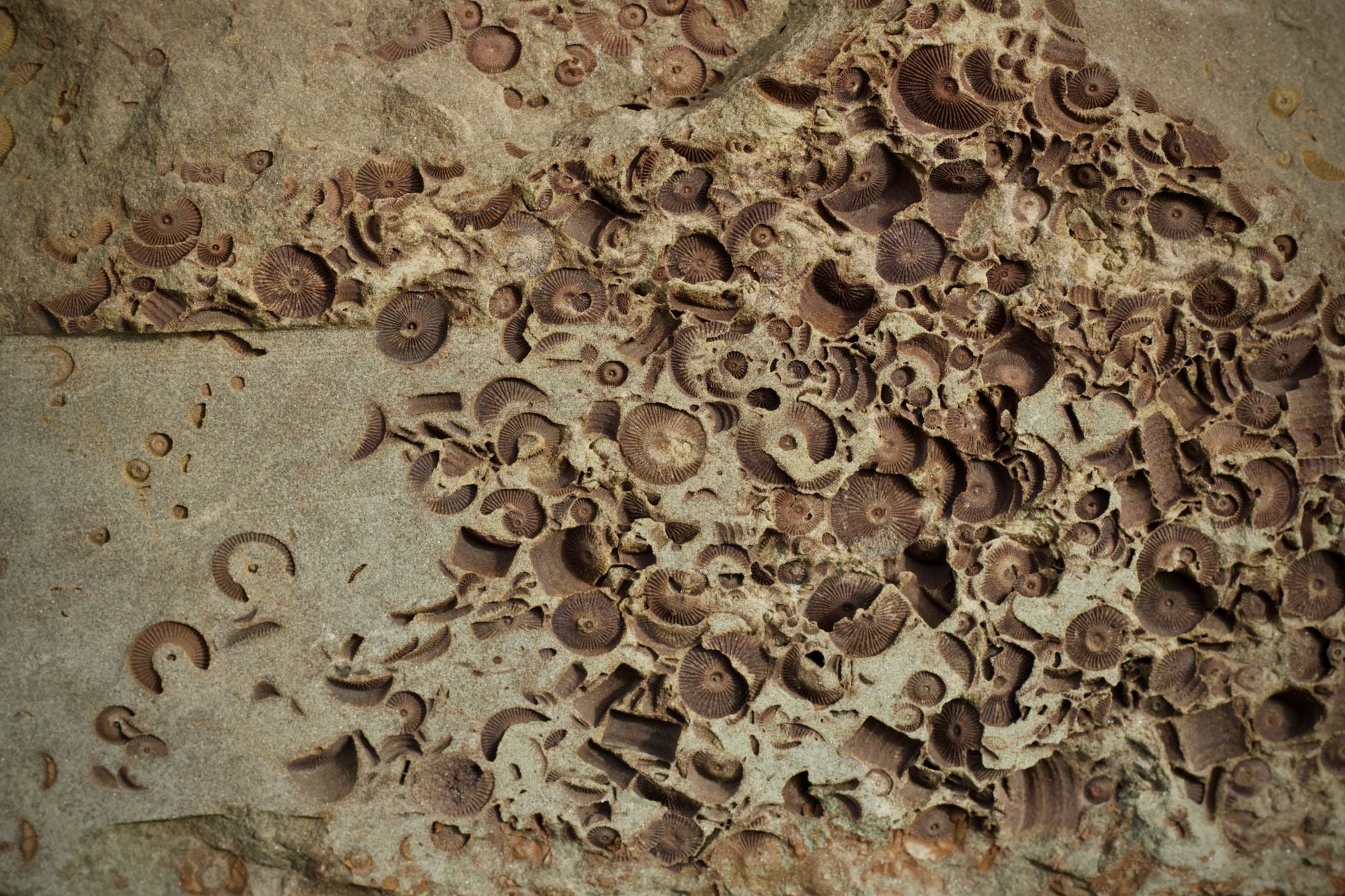
The history of life is full of disappearances, but they are not spread evenly through time. Long intervals of comparatively modest turnover are interrupted by sharp pulses in which extinction accelerates across many groups at once.
That uneven pattern allowed palaeontologist David Raup to construct what he called a “kill curve”. His analysis suggested that an event eliminating at least 10 per cent of species occurs, on average, about once every million years. Raise the loss to around 30 per cent and the mean interval becomes about 10 million years. At roughly 65 per cent, it stretches to about 100 million years.
Those figures sound like a timetable.
They are not.
The intervals describe the average frequency of differently sized extinction episodes in the fossil record. They do not say that catastrophes arrive regularly, identify what causes them or reveal how long remains until another one. Two large crises could occur unusually close together, followed by a much longer quiet interval.
How scientists built a curve from vanished life
Raup’s 1991 paper in the journal Paleobiology began with a compilation assembled by fellow palaeontologist Jack Sepkoski. It recorded the stratigraphic ranges of 17,621 genera of marine organisms across roughly 600 million years.
A stratigraphic range runs from a group’s first known appearance in the rock record to its last. Raup used the distribution of those ranges, together with survivorship analysis and simulations, to estimate how extinction risk at the species level must have varied through time.
The answer was highly uneven. A typical species faced very low extinction risk during most short intervals, while occasional pulses carried much greater risk. Combining those quiet periods and crises into a single average obscured the pattern.
The kill curve instead linked the magnitude of an episode to its mean waiting time. Small losses were common. Severe losses were rare. The 10, 30 and 65 per cent figures are convenient points read from a continuous curve, not boundaries separating three natural classes of disaster.
This also challenged a simple division between “background” and “mass” extinction. In Raup’s reconstruction, the events formed a long, skewed distribution rather than two clearly separated categories. The famous Big Five occupied its extreme tail.
What a mean waiting time really means
A mean waiting time is calculated by looking across a long record and asking how frequently events of at least a given size occurred. It is similar to the return periods used for floods or earthquakes, although extinction episodes need not follow the same statistical rules as either.
A 100-million-year mean interval does not produce a 100-million-year cycle. It certainly does not mean risk stays low for 99 million years and then suddenly becomes unavoidable.
Earth’s major extinction crises have not been copies of one another. The end-Cretaceous event 66 million years ago was driven by an asteroid impact whose effects were amplified by the rocks it struck. SpaceDaily has examined how sulphur-rich material at the impact site helped turn the collision into a global climate disaster.
The much larger end-Permian crisis followed immense volcanism, greenhouse warming and severe disruption of ocean chemistry. Recent work has strengthened the case that warming and oxygen loss combined to make marine habitat physiologically inaccessible to many animals.
Other crises involved rapid cooling, sea-level change, ocean acidification, anoxia and ecological cascades in different combinations. A curve describing their sizes cannot turn those distinct causes into a single clock.
The fossil record has limits
Raup’s curve was a major attempt to convert an incomplete record into a species-level risk distribution. Its numbers should still be treated as estimates rather than universal constants.
Fossilisation is selective. Marine animals with hard shells and skeletons are far more likely to be preserved than soft-bodied organisms, many terrestrial species or life in environments where sediments do not accumulate. Sampling also varies with the amount of rock available, the places palaeontologists have searched and the precision with which layers can be dated.
The original data mostly tracked genera, not species. Inferring species losses from genus ranges requires assumptions about typical diversity and survival within each genus. Short pulses may also appear spread across a longer interval because fossils are rare and geological dates carry uncertainty.
Raup therefore presented uncertainty bounds around the curve and stressed that it was a description of the record. It did not establish any cause of extinction.
Newer occurrence-level databases have allowed researchers to revisit the old patterns with better corrections for sampling. A later synthesis of marine fossil data found no autocorrelation in extinction rates and no convincing spectral evidence for a regular long-term cycle. Some researchers continue to argue for periodic components in the record, but no proposed cycle functions as a dependable forecast.
Extinction is clustered, not steadily accumulated
The kill curve’s most important message is not its three memorable recurrence figures. It is that extinction risk varies enormously.
If individual species simply vanished independently at a constant rate, losing 10 per cent of all species during the same short interval would be extraordinarily unlikely. The fossil pattern instead shows clustering. Environmental shocks can strike many lineages at once, while the removal of habitats or ecologically important groups can trigger further losses.
Even so, the Big Five account for only a small share of all extinction through the Phanerozoic, roughly 5 per cent in Raup’s calculation. Most vanished species disappeared during smaller pulses and quieter turnover that never received a mass-extinction label.
This is why an average background rate can be misleading. It blends long stretches of low risk with brief intervals of extreme danger, much as an annual rainfall average can hide both drought and flood.
There is no protection in not being due
The lack of a geological countdown does not make present-day biodiversity loss less serious.
The 2019 global assessment by the Intergovernmental Science-Policy Platform on Biodiversity and Ecosystem Services concluded that human actions threaten more species with extinction than at any previous point in human history. It estimated that around one million species face extinction, many within decades, unless the pressures are reduced. It also assessed the current extinction rate as at least tens to hundreds of times the average over the past 10 million years.
Those estimates carry substantial uncertainty because most living species have not been formally assessed and many have not even been described. Nor has humanity yet erased 65 or 75 per cent of all species, the scale associated with the most severe crises in deep time.
What has changed is the rate and reach of the pressures. Habitat conversion, direct exploitation, climate change, pollution and invasive species are operating simultaneously around the world. Their effects depend on human decisions, not the elapsed time since the last asteroid impact or volcanic catastrophe.
The fossil record offers a distribution of what happened before. It cannot provide an appointment for what happens next.
There is no mass-extinction clock to reset, and no safe interval guaranteed between crises.