Ninety-six hours of MeerKAT data recorded during the telescope's 2018 commissioning have produced the first interferometric detection of neutral hydrogen's own power spectrum, measured without cross-correlating the hydrogen maps against a galaxy survey

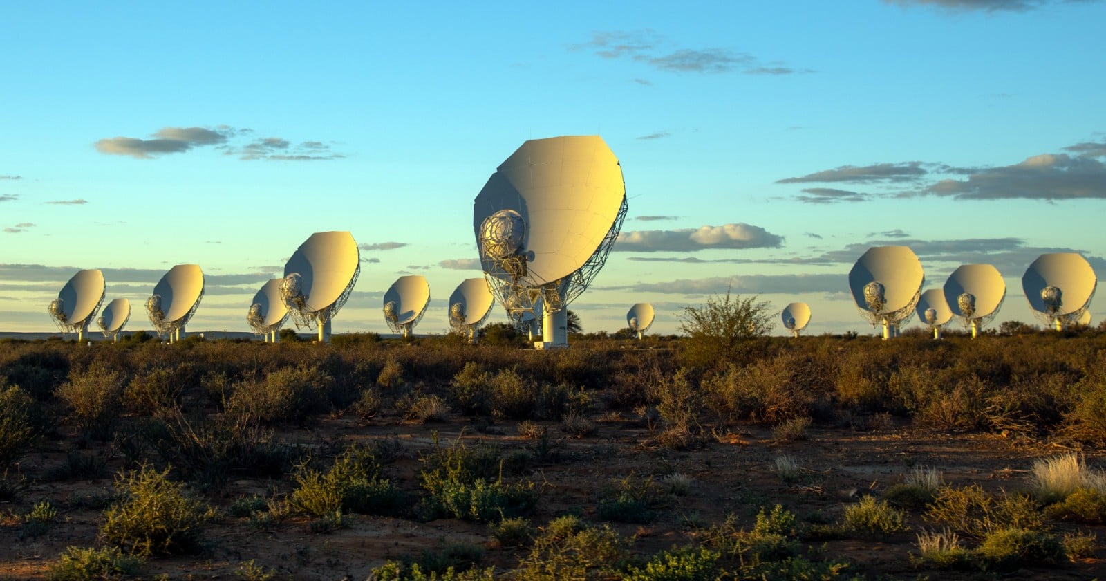
The MeerKAT array in South Africa was still being commissioned in 2018. Over nine sessions between 30 June and 4 November that year, using between 58 and 62 of its 64 dishes, it collected about ninety-six hours of data on DEEP2, a field already used to produce what the paper calls the deepest radio source count to date. The visibilities went into the South African Radio Astronomy Observatory archive under proposal ID SCI-20180426-TM-01, and the uncalibrated visibilities remain public.

Eight years later those same ninety-six hours have produced a detection of the cosmological power spectrum of neutral hydrogen at two redshifts, roughly 0.32 and 0.44, measured from the radio data alone. The result was published in July in The Astrophysical Journal Letters by Sourabh Paul, Zhaoting Chen, Mario G. Santos and Laura Wolz. Detections of this signal had previously been achieved only by cross-correlating hydrogen maps against galaxy surveys.

A single line under a loud sky

Neutral hydrogen announces itself at a single radio frequency. The hyperfine transition of the hydrogen atom emits at 1420 MHz in its own rest frame, and because the universe has been expanding, hydrogen further away arrives at lower frequencies. Light collected at 1077.5 MHz comes from gas at a redshift of about 0.32; at 986 MHz the redshift is about 0.44. The Inter-University Institute for Data Intensive Astronomy describes that light as coming from a period when the universe was several billion years younger than it is today.

The signal is extraordinarily faint. Hydrogen surveys that pick out galaxies one at a time have historically been stuck below redshift 0.1. Intensity mapping is the workaround: instead of resolving individual galaxies, it averages the collective emission from many unresolved ones and treats the brightness fluctuations as a tracer of where the matter is.

It carries a foreground problem. The galaxy we live in is a bright radio object, and so are the radio galaxies behind it, and both drown out the hydrogen. Previous teams got around this by cross-correlating their hydrogen maps against galaxy surveys, on the reasoning that systematic errors in radio data should not correlate with measurements at entirely different wavelengths. The Green Bank Telescope made the first such detection, Parkes followed, and the CHIME interferometer later made a stacking detection over a wide area. The trick works. It also requires the galaxy survey.

The modes where the foregrounds live

Paul and colleagues used foreground avoidance instead. The method exploits the fact that foregrounds and signal behave differently across frequency: the Milky Way’s synchrotron glow and the radio galaxies are smooth across the band, while the hydrogen signal is not. Fourier transforming along the frequency axis piles the smooth components up at short delays, in a region known as the wedge, and none of that region is used.

Where the boundary is drawn decides how much data survives. MeerKAT’s beam is about a degree across, which alone would put the line at a line-of-sight mode roughly 0.02 times the transverse one. On the most extreme assumption, that bright sources leak in through the sidelobes from anywhere on the sky, it moves to 0.26. The team drew it at 0.3, discarding more than even that case required.

They also split the data in two. Visibilities from odd-numbered scans went into one cube and even-numbered scans into another, and the power spectrum was computed by cross-correlating the two. Because the thermal noise in one time block is independent of the other’s, that cross-correlation removes the noise bias instead of requiring it to be subtracted, and suppresses anything varying with time.

Interference that survived the pipeline

The standard processing had already discarded two frequency bands outright for persistent interference, and flagged about a tenth of what remained within the range of baselines this analysis uses. Excess power showed up anyway. In the two-dimensional power spectrum it appears as stripes near the horizon boundary the team had drawn. Tracing it back, they found that the fraction of contaminated delay modes rises sharply near the zero point of one baseline coordinate, which is a fingerprint: baselines near zero get less smearing from the Earth’s rotation, so faint broadband interference that would otherwise wash out stays coherent there. The paper notes this has been seen in MeerKAT data before. The pipeline missed it; the community had not.

The team went looking for a culprit. Wide-field images out to the horizon identified no localised horizon source, persistent or transient, that correlated with the contamination. Their own reading is that this disfavours a single dominant localised emitter without ruling out extremely faint, intermittent or spatially distributed interference. Follow-up in fringe-rate space put the anomalous power close to zero fringe rate, pointing at something terrestrial or at coupling between the dishes, not at anything on the sky.

So they built two ways of removing it, and the result splits in two.

Why the cleaning method changes the confidence level

The first, baseline flagging, examines the delay spectrum of every antenna pair averaged over each fifteen-minute scan, and throws out the whole pair for that scan if a peak rises more than five sigma above the expected thermal noise outside the foreground wedge. It is blunt and familiar, and it operates well before the power spectrum is computed. It yields a detection at 3.2 sigma at redshift 0.32 and 3.5 sigma at redshift 0.44.

The second flags later and more surgically. After the visibilities have been gridded and transformed, it compares each three-dimensional pixel against a thermal noise simulation and discards the pixel if it deviates by more than five sigma. About one per cent of pixels in the usable window get cut. Because it removes contaminated modes instead of whole antenna pairs, far more data survives, and the significance rises to 5.9 sigma at redshift 0.32 and 9.18 sigma at redshift 0.44. Those are the figures with the first two wavenumber bins excluded, which is how the paper’s abstract quotes them; including those bins the numbers are 6 and 9.3 sigma.

So the cost of the blunter method is 3.2 against 5.9 at the lower redshift and 3.5 against 9.18 at the higher one. The paper’s explanation is not that the surgical method finds more signal but that the blunt one throws away sensitivity: in the dense core of the array, where most of the measurement lives, baseline flagging discards more than half the available data on average, and the authors attribute the lower significance primarily to the resulting rise in the thermal noise floor rather than to any suppression of signal amplitude.

That leaves a reasonable objection to the surgical method, which the authors put themselves. Flagging that happens so close to the final measurement risks forcing the data to match the distribution it is being compared against. Their defence: the threshold is drawn from noise simulations calibrated against Stokes V data, noise dominates the hydrogen signal in every pixel anyway, and simulations show the signal loss from the cut is negligible. Against their fiducial five sigma, a ten sigma cut gives a reduced chi-squared of 0.45 and a three sigma cut gives 0.33, while doing no flagging at all gives 28.

Their most diagnostic check is a null test. The contaminating interference is broadband, and they demonstrate it: on a contaminated baseline, the excess appears at the same physical delay in both frequency windows, with a correlation coefficient of 0.93 between them. The cosmological signal, by contrast, should be completely uncorrelated between two different redshifts. So they cross-correlated the two redshift bins against each other. Had the flagging been failing, a contaminant coherent across both bands would have produced a spurious signal. They report no significant correlation, and the same test run on the baseline-flagged data also comes back consistent with zero. A jackknife test dropping one observing block at a time is likewise coherent.

Where the paper’s own numbers get soft

The measurement pins down very little astrophysics. The team fitted a halo model to the power spectrum and most of the parameters did not converge. Without an external prior the posterior on the cosmic hydrogen density is broad enough to reach about ten to the minus five, far below established measurements, and the velocity dispersion posterior at the lower redshift runs into the edge of the prior the team imposed at 500 kilometres per second.

Feeding in existing hydrogen density measurements, from stacking at the lower redshift and damped Lyman alpha systems at the higher one, fixes that parameter by construction and does not visibly improve the shot noise or the velocity dispersion. At the higher redshift the density profile parameter and the slope of the halo occupation do start to come under control. The paper reports a mild one-sigma tension between those priors and its own unconstrained posterior, and names two candidate causes: the simplicity of the halo model, or signal loss that has not been corrected for. The scales measured here sit where shot noise and velocity dispersion dominate, which carry little information about the overall hydrogen abundance.

The paper also contains a number that disagrees with itself. Its detailed sections quantify the calibration errors at roughly 0.1 per cent, and separately put the bandpass error below ten to the minus three on the gridded data; the summary describes the calibration as accurate to about ten to the minus five. Those are two orders of magnitude apart. The detailed sections carry the derivation, so that is the figure to trust, and anyone quoting the summary instead will be off by a hundredfold.

The amplitude and what follows it

Stripped of the modelling, the measurement is a statement about how clumpy the hydrogen is. At a scale of one megaparsec the team puts the root-mean-square fluctuation at 0.44 plus or minus 0.04 millikelvin at redshift 0.32, and 0.63 plus or minus 0.03 millikelvin at redshift 0.44, from eight thousand bootstrap realisations. A 2021 forecast by the same lead author had estimated that roughly a hundred hours of MeerKAT time should be enough for a statistical detection; ninety-six hours of commissioning data came in just under that.

The power spectrum amplitude runs around one millikelvin squared times a cubic megaparsec at the larger scales and about a tenth of that at the smaller ones, which the authors say is in line with expectations. How much that agreement establishes is a separate question: by the paper’s own account the predicted signal at these scales spans an order of magnitude in the main text and several in the appendix, depending on modelling choices, which leaves a wide target to hit.

More data exists. The MIGHTEE and Laduma surveys are taking deep MeerKAT observations on fields suited to this kind of analysis, and with a higher signal-to-noise ratio the power spectrum could be binned in two dimensions instead of one, preserving the line-of-sight information that would break the degeneracy between velocity dispersion and shot noise. MeerKAT is a precursor to the Square Kilometre Array, and the paper closes by pointing at the next generation of radio telescopes generally: faint broadband interference that survived a standard flagging pipeline was strong enough to contaminate the very window this measurement lives in. Whether the next generation of radio telescopes can measure hydrogen precisely enough to constrain cosmology may depend less on the telescopes than on how quiet the ground underneath them can be kept.